Overview and motivation
Figure 1
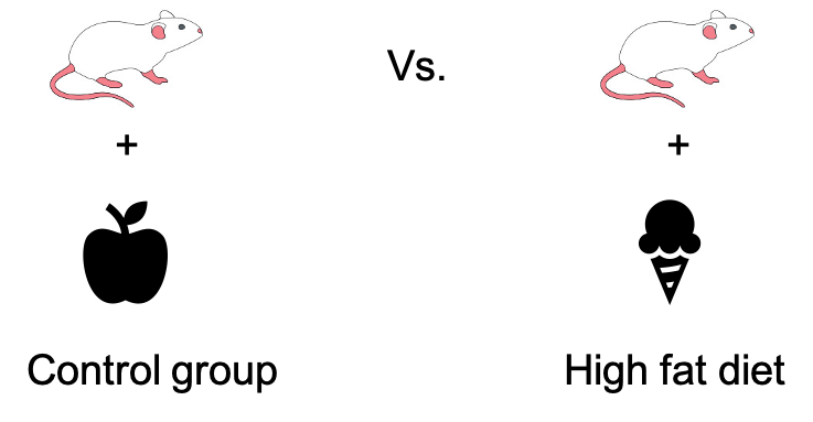
Mice with different diets
Figure 2
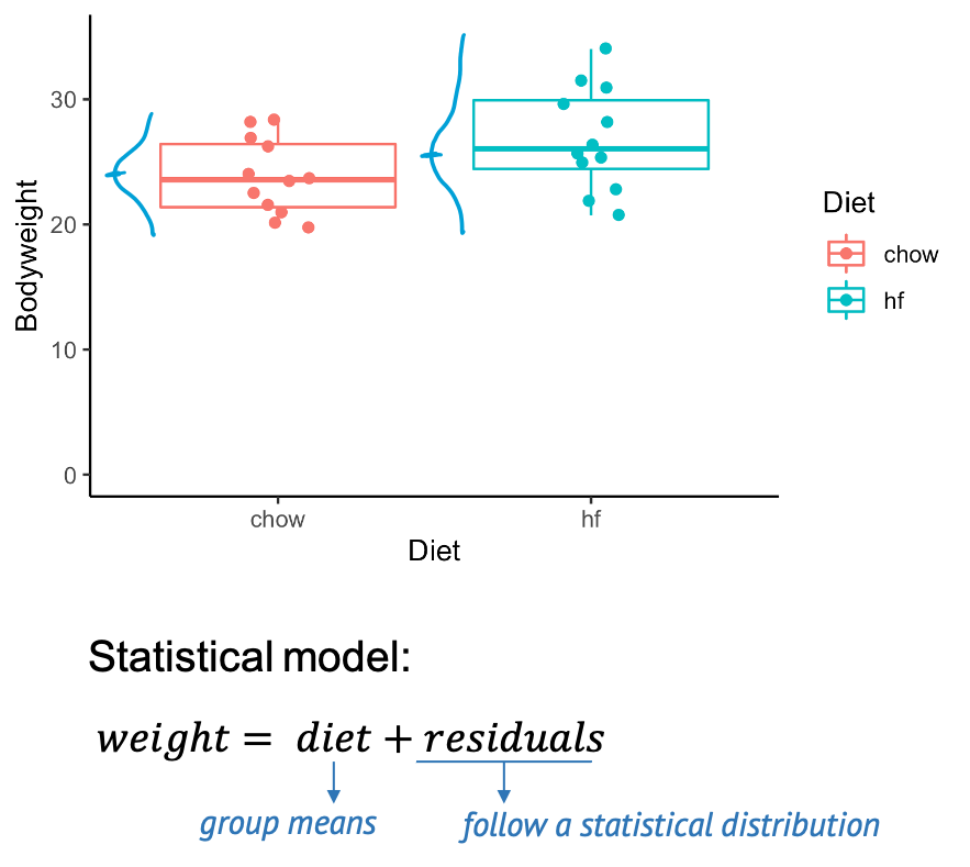
Does the diet affect the mice’s weight?
Our first test: Disease prevalence
Figure 1
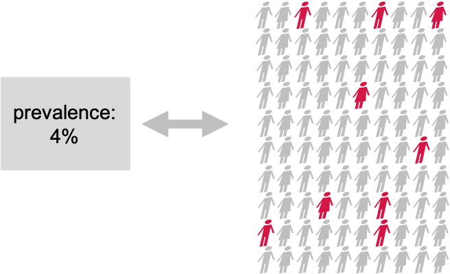
Example: Disease prevalence
Figure 2
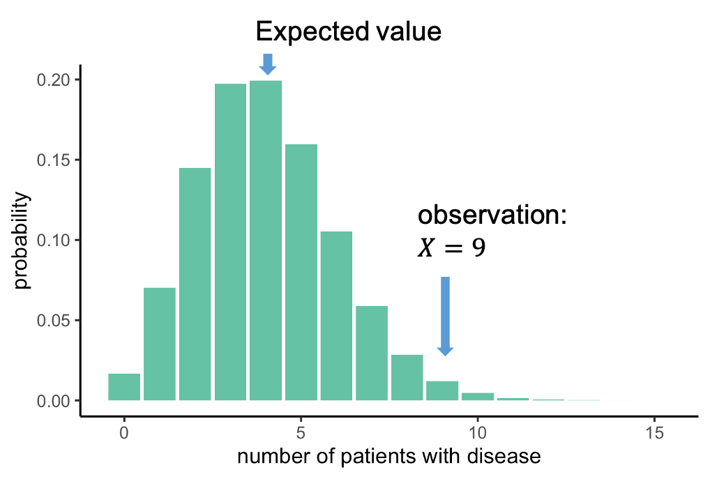
The null distribution
Figure 3
The null distribution
Figure 4

Please take a minute…
One-sided vs. two-sided tests, and data snooping
Figure 1
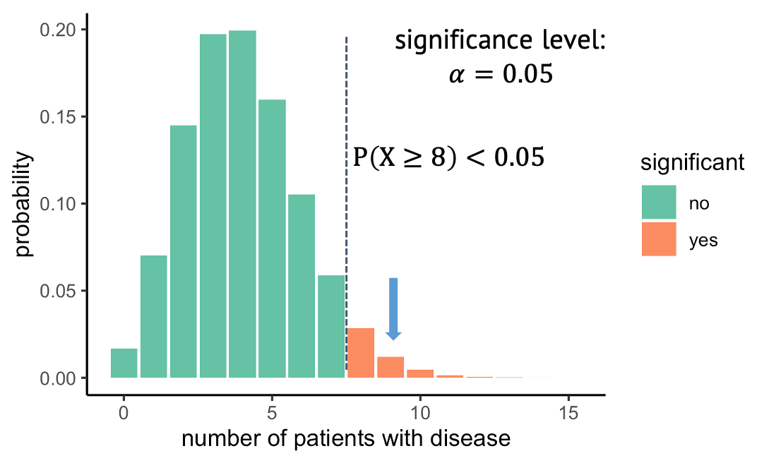
One-sided test
Figure 2
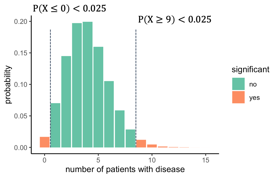 We should look on both sides of the distribution and ask
what outcomes are unlikely. For this, we split the 5% significance to
2.5% on each side. That way, we will reject everything below 1, or above
8. The alternative hypothesis is now that the prevalence is different
from 4%.
We should look on both sides of the distribution and ask
what outcomes are unlikely. For this, we split the 5% significance to
2.5% on each side. That way, we will reject everything below 1, or above
8. The alternative hypothesis is now that the prevalence is different
from 4%.
Errors in hypothesis testing
Figure 1
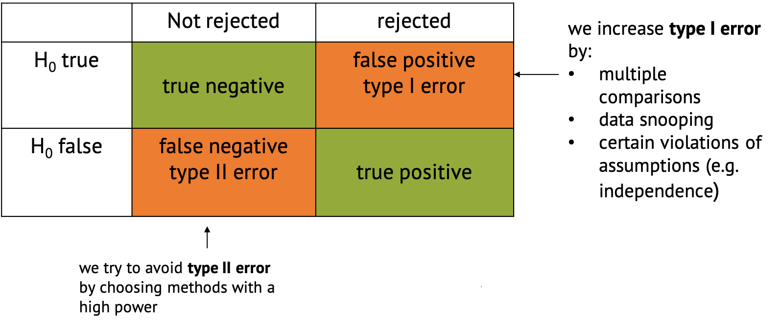
Errors in hypothesis testing
One-sample t-test
Figure 1
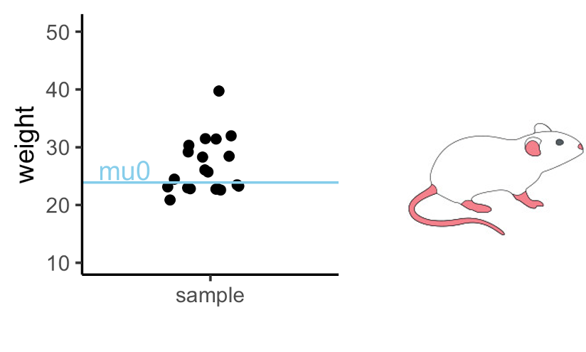
Scenario for one-sided t-test: Comparing mouse
weights to a single value.
Figure 2
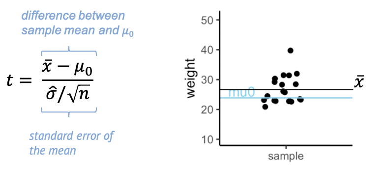
The t-statistic is a scaled difference between
sample mean and \(\mu_0\)
Figure 3
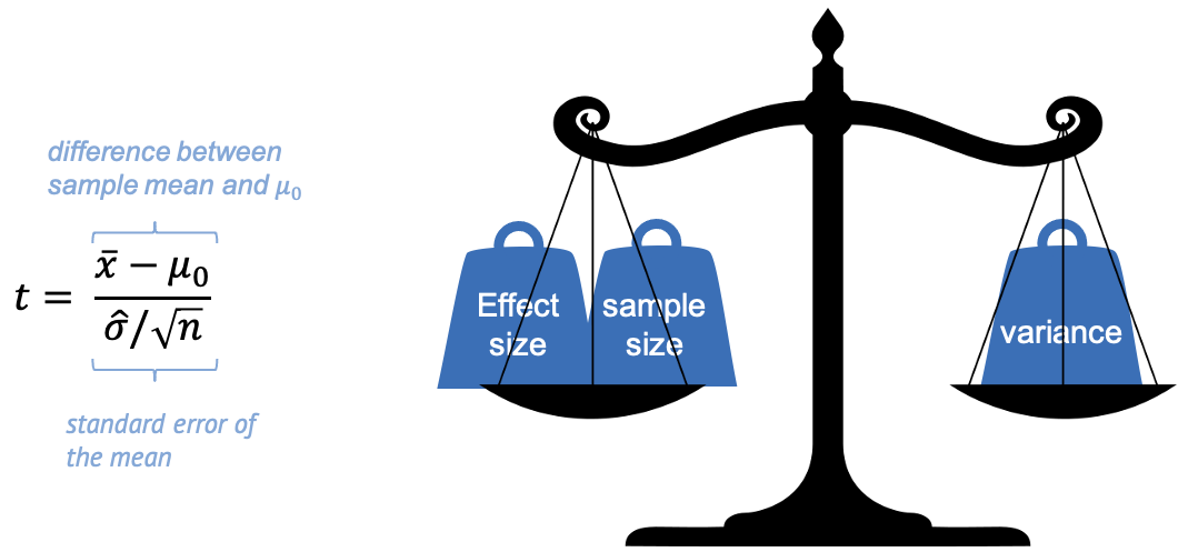
The t-statistic weighs effect size and sample
size against variance.
Figure 4
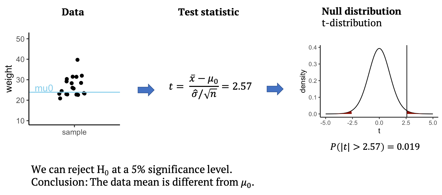
One-sample t-test
The distribution of t according to the Central Limit Theorem
Figure 1

The distribution of t in practice
Figure 1
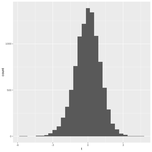
Figure 2
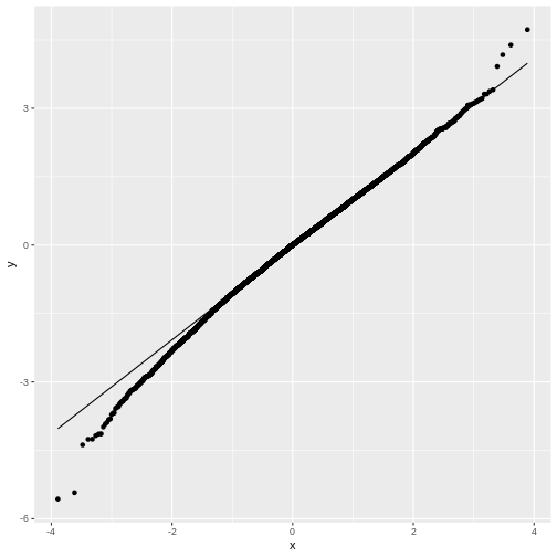
Figure 3
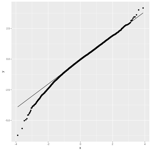
Figure 4

The t distribution for different degrees of
freedom (wikipedia)
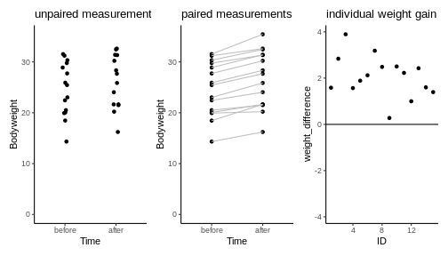
The two-sample and paired t-test
Figure 1
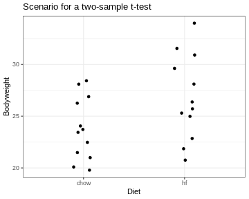
Figure 2

Figure 3
Interpreting p-values
Figure 1
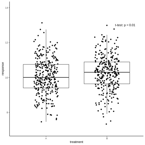
Figure 2
Have a coffee! (Image: Wikimedia)
Summary and practical aspects
Figure 1

Cookbook (image adapted from kindpng.com)
Figure 2

In practice (image adapted from
kindpng.com)