Types of errors and error rates
Last updated on 2025-01-14 | Edit this page
Overview
Questions
- What are false positives and false negatives and how do they manifest in a confusion matrix?
- What are some of real examples where false positives and false negatives have different implications and consequences?
- What are type I error rates?
Objectives
- Understand the concept of false positives and false negatives and how they are represented in a confusion matrix
- Analyse and discuss scenarios where false positives and false negatives pose distinct challenges and implications
- Highlight situations where minimizing each type of error is crucial
Types of errors
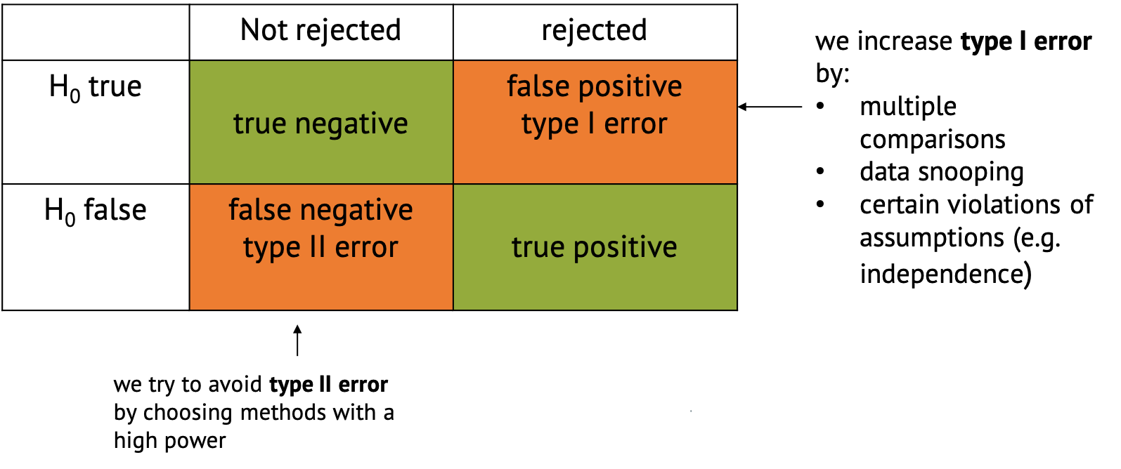
In hypothesis testing, the evaluation of statistical significance involves making decisions based on sampled data. However, these decisions are not without errors. In this tutorial, we will explore the concept of errors in hypothesis testing (Type I and Type II errors), and their implications.
Type I Error
A type I error occurs when we reject a null hypothesis that is actually true. For example, in our previous example where we conducted many similar experiments, we experienced type I error by concluding that exposure to air pollution has an effect on disease prevalence (rejecting the null hypothesis) when it actually has no effect. Type I errors represent false positives and can lead to incorrect conclusions, potentially resulting in wasted resources or misguided decisions.
Type II Error
A type II error occurs when we fail to reject a null hypothesis that is actually false. For example, when we fail to conclude that exposure to air pollution has an effect on disease prevalence (failing to reject the null hypothesis) when it actually has a positive effect. Type II errors represent false negatives and can result in missed opportunities or overlooking significant effects.
Type II errors often occur when in settings with low statistical power is chosen. Statistical power refers to the probability of correctly rejecting the null hypothesis when it is indeed false. In simpler terms, it measures the likelihood of detecting a true effect or difference if it exists. Low power can be due to properties of the sample, such as insufficient number of data points, or high variance. But there are also tests that are better at detecting an effect than others in certain settings.
Confusion Matrix
In the context of hypothesis testing, we can conceptualize Type I and Type II errors using a confusion matrix. The confusion matrix represents the outcomes of hypothesis testing as True Positives (correctly rejecting H0), False Positives (incorrectly rejecting H0), True Negatives (correctly failing to reject H0), and False Negatives (incorrectly failing to reject H0).

Implications of type I and type II errors
In hypothesis testing, the occurrence of Type I and Type II errors can have different implications depending on the context of the problem being addressed. It is crucial to understand which errors are problematic in which situation to be able to make informed decisions and draw accurate conclusions from statistical analyses.
Type I errors are particularly problematic in situations where the cost or consequences of incorrectly rejecting a true null hypothesis are high. Again, if we refer back to our example, if we incorrectly conclude that there is a significant difference in disease rates between the test groups exposed to air pollution and the average for the whole population when, in fact, there is no such difference, it could lead to misguided policies or interventions targeting air pollution reduction. For instance, authorities might implement costly environmental regulations or public health measures based on erroneous conclusions. In this case, the consequences include misallocation of resources, leading to unnecessary financial burdens or societal disruptions. Moreover, public trust in scientific findings and policy decisions may be eroded if false positives lead to ineffective or burdensome interventions.
Type II errors are problematic when failing to detect a significant effect has substantial consequences. If we fail to detect a significant difference in disease rates between the test group and the population average when there actually is a difference due to air pollution exposure, it could result in overlooking a serious public health concern. In this case, individuals living in polluted areas may continue to suffer adverse health effects without receiving appropriate attention or interventions. The consequences include increased morbidity and mortality rates among populations exposed to high levels of air pollution. Additionally, delayed or inadequate response to environmental health risks may exacerbate inequalities in health outcomes.
An example of cancer screening
Cancer screening exemplifies a medical testing paradox, where the interpretation of test results can be influenced by factors such as disease prevalence, test sensitivity, and specificity.
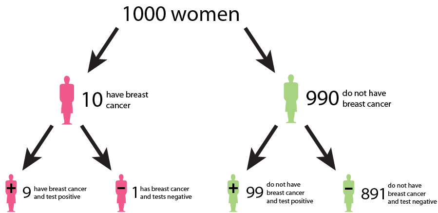
Let us say that in a sample of 1000 women, 1% (10) have cancer, while the remaining 99% (990) do not have cancer. This gives us the prevalence of a disease. However, after testing, the test results show that out of the 10 women with cancer, 9 receive a true positive result (correctly identified as positive), and 1 receives a false negative result (incorrectly identified as negative). False negatives can delay the diagnosis and treatment of cancer, allowing the disease to progress unchecked and potentially reducing the effectiveness of treatment options. This can result in poorer outcomes and decreased survival rates for patients. In addition, out of the 990 women without cancer, 89 receive false positive results (incorrectly identified as positive), and 901 receive true negative results (correctly identified as negative). False positive can lead to unnecessary follow-up tests, procedures, and treatments for individuals who do not have cancer. It can cause anxiety, physical discomfort, and financial burden for patients, as well as strain on healthcare resources.

We could interpret that:
The probability that a woman who receives a positive result actually has cancer is ≈ 1/10 ( 9/ (9 + 89)). This is the positive predictive value (PPV) of the test.
The sensitivity of the test, which measures its ability to detect the presence of disease is 90% (9/10 * 100). This means that the false negative rate of the test is 10%.
The specificity of the test, which measures its ability to correctly identify individuals without the disease is ≈ 91% (901/990 * 100). Here, the false positive rate of the test is 9%.
While the test may have high accuracy in terms of sensitivity and specificity, the positive predictive value is relatively low due to the low prevalence of the disease in the population. This means that a positive result from the test does not strongly predict the presence of the disease in an individual. Similarly, false positives and false negatives can affect the negative predictive value of the test, which measures its ability to correctly identify individuals who do not have cancer. False negatives decrease the negative predictive value, while false positives increase it, potentially leading to misinterpretation of test results.
This example underscores the complexity of interpreting medical test results and emphasizes the need to consider factors such as disease prevalence, test sensitivity, and specificity in clinical decision-making. Increasing sensitivity may reduce false negatives but can also increase false positives, and vice versa. Thus, optimizing the trade-off between sensitivity and specificity is crucial to minimize false positives and false negatives while maximizing the accuracy of the screening test.
What do we learn?
In many real-world scenarios, there is a trade-off between Type I and Type II errors, and the appropriate balance depends on the specific goals and constraints of the problem. Reseachers may prioritize one over the other based on the severity of the consequences. For example, in cancer screenings, minimizing false negatives (Type II errors) is typically prioritized to avoid missing potential cases of cancer, even if it leads to an increase in false positives (Type I errors).
Effective evaluation of Type I and Type II errors necessitates a comprehensive consideration of the associated costs, risks, and ethical implications. This holistic approach enhances the validity and reliability of research findings by ensuring that decisions regarding hypothesis acceptance or rejection are informed not only by statistical significance but also by the potential real-world consequences of both false positives and false negatives. By carefully weighing these factors, researchers can make informed decisions that minimize the likelihood of erroneous conclusions while maximizing the practical relevance and ethical soundness of their findings.
Error rates
In the following chapters, we’ll see different methods that all aim to control for false positives in different settings.
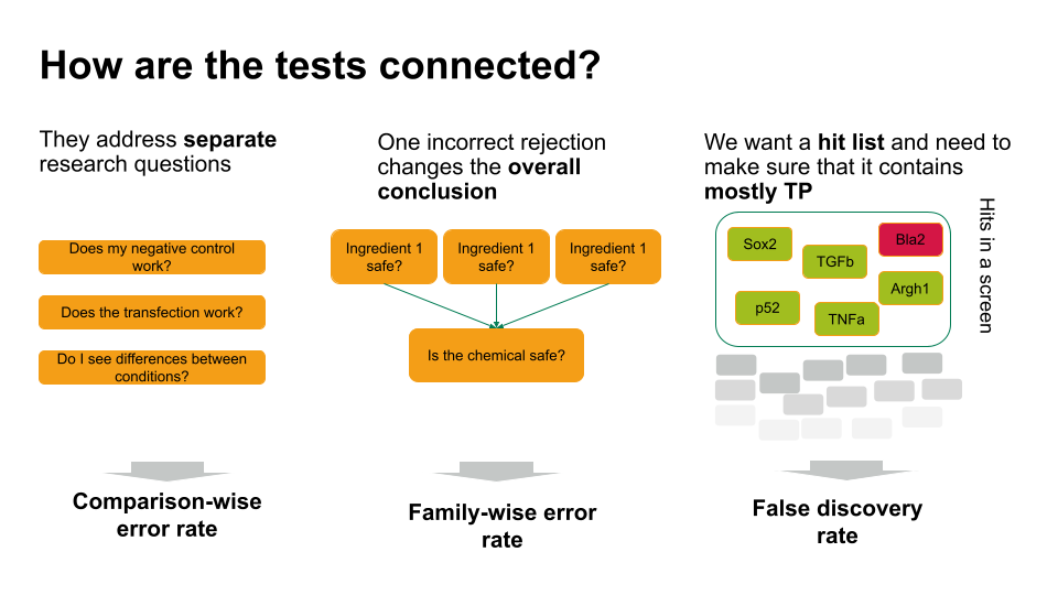
The main distinction between these methods lies in the error rate that they control for. We’ll get to know three error rates:
- The comparison-wise error rate, where we use the p-value as we obtain it from each individual test (no correction).
- The family-wise error rate, where we like to avoid any false positives.
- The false-discovery rate, where we like to control the fraction of false positives within our hits.
We’ll see screening scenarios and multiple comparisons, and in both settings, different methods exist to control for the different error rates.
The plethora of methods can often be overwhelming. Therefore it’s good to keep in mind that in practice, most of the time the workflow can be broken down into three simple steps:
- Clearly define your research question, and describe
the testing scenario.
- Based on your research question, choose an appropriate error rate that you need to control for.
- Choose a method that controls for the selected error rate that applies for the testing scenario at hand.
Choosing the error rate is often a philosophical question. Before we dive into the details of the individual methods, let’s get an overview on the three error rates we’re considering. Which one to choose depends on how the hypothesis tests in your scenario are connected.

- If each of these tests answers a separate research question, you can apply the comparison-wise error rate, which means you don’t have to correct anything.
- Sometimes, one incorrect rejection changes the overall conclusion in your research setting. For example, if you decide on the safety of a chemical, which is a mixture of ingredients. You can ask for each ingredient whether it’s safe (null hypothesis: it’s safe). If all null hypohteses are true (all ingredients are safe), you’d like to conclude that the entire chemical is safe. However, if you falsely reject one individual null hypothesis, this will change the overall conclusion (you falsely call the chemical unsafe). Therefore, you’d like to control the probability of making any false rejections, which is called the family-wise error rate.
- In many scenarios, a few false positives won’t change the overall conclusion. For example, in biological screens, we aim for a hit list of candidate genes/proteins/substances that play a role in a process of interest. We can then further verify candidates, or identify pathways that are over-represented in the hits. For this, we can live with a few false positives, but we’d like to make sure that most of what we call a hit, actually is a hit. For such scenarios, we control for the false discovery rate: the percentage of false positives among the hits.
