What is multiple testing
Last updated on 2024-07-16 | Edit this page
Overview
Questions
- What is multiple testing?
Objectives
- Define multiple testing
What is multiple testing
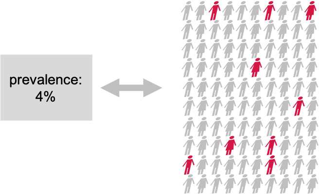
Suppose the prevalence of a disease in the general population is 4%. In this population, lives a group of individuals who have all been exposed to air pollution. Concerned about their health, we decide to embark on a quest to uncover whether being exposed to air pollution influenced the risk of contracting this disease.

Setting the null and alternative hypothesis
We would like to conduct a hypothesis test to find out whether the prevalence in the test group differs from the known 4%.
Null Hypothesis (\(H_0\))
The prevalence of the disease within test group exposed to air pollution is the same as the known prevalence in the general population (4%). This means that the proportion of individuals exposed to air pollution in the test group who have the disease is also 4%.
Alternative Hypothesis (\(H_1\))
The prevalence of the disease within the test group exposed to air pollution is different from the known prevalence in the general population. This means that the proportion of individuals exposed to air pollution in the test group who have the disease is either higher or lower than 4%.
Data collection and testing
We assemble a group of 100 individuals who have been exposed to air pollution (test group) from the population and each individual is carefully examined, checking for any signs of the disease. Out of the 100 individuals, we discover that 9 of them were indeed suffering from the disease, so the observed proportion is 9%. This is different from 4%, but we are not satisfied with just this knowledge, since the observed difference in proportions could be due to chance. We want to know if this prevalence of the disease within the group exposed to air pollution was significantly different from the population’s average, meaning that it’s very unlikely to observe this difference just by chance. So, we decide to perform binomial test (please refer back to binomial tests tutorial) The binomial distribution. With this test, we could compare the observed prevalence within our group that has been exposed to air pollution to the known prevalence in the entire population.
We set our significance level (α) beforehand, typically at 0.05, to determine whether the results are statistically significant.
R
#For known parameters (n=100, p=0.04), we calculates the the chances of getting the 9 individuals that indeed suffered from the disease.
n = 100 # number of test persons
p = 0.04 # Known prevalence of the disease in the general population
dbinom(x=9, size=n, prob=p)
OUTPUT
[1] 0.01214746The P-value we get, is the probability of obtaining extreme outcome, assuming that the null hypothesis is true. Therefore, the binomial test calculates the probability of observing the obtained (9 persons with a disease) or more extreme results assuming the null hypothesis is true. If this probability is sufficiently low (below our chosen significance level), we reject the null hypothesis in favor of the alternative hypothesis.
The binomial test result (~0.012) reveals that the prevalence of the disease among the individuals exposed to air pollution was indeed significantly different from that of the population.
What if we did many similar experiments?
Conducting a single study might not provide conclusive evidence due to various factors such as sample variability, random chance, and other unknown influences.
We decide to investigate the potential impact of air pollution on disease prevalence in 200 various locations. We want to assess whether there is a significant difference in disease rates between groups exposed to air pollution and the average for the whole population.
We want to know how hypothesis testing works, when we perform it simultaneously or in quick succession on many tests.
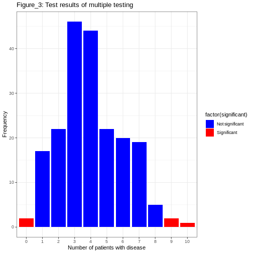
We therefore decide to simulate the scenario where we conduct 200 tests, each with a 5% chance (alpha = 0.05) of producing a significant result (i.e., a p-value less than 0.05) even when the null hypothesis is true.
Our null hypothesis in each location is that there is no real difference in disease rates between the groups exposed to air pollution and the average for the whole population.

To do this, we write a program in R, which simulates study results when the prevalence in the test group is 4% (null hypothesis is true). We run these experiments to see what would happen if we kept doing tests even when there was not actually any difference.

We are interested in determining if the observed proportion significantly deviates from the expected proportion (0.4) in either direction (either higher or lower). As this is a two-tailed binomial test, we needed to adjust the bounds for what is considered “significant” based on the significance level of 0.05. We are interested in the extreme tails of the distribution that contain 2.5% of the data on each side.
We therefore use qbinom() function in this simulation to
calculate the quantiles of the binomial distribution corresponding to
the 2.5th and 97.5th percentiles. This gives us the bounds that would
contain 95% of the data under the null hypothesis. We then classify a
group as “significant” if the observed number of patients falls below
the 2.5th percentile or above the 97.5th percentile of the binomial
distribution.
In the resulting histogram, we find that even in a world where there was no true difference in disease prevalence, about 5% of our simulated experiments yielded statistically significant results purely by chance (the red bars).
It is important to note that the significance level (α) that we choose for each individual test directly impacts the rate of false positives. This is basically the Comparison-Wise Error Rate (CWER), the probability of making a Type I error (false positive) in a single hypothesis test. In our example, we have set α=0.05 for each individual test, which means we are essentially saying that we are willing to accept a 5% chance of making a false positive error for each test, and this means that for 100 tests, we expect about 5 false positives.
By running this simulation multiple times, we can observe how often we get false positive results when there should be none. This helps us understand the likelihood of obtaining a significant result purely by chance, even if there is no true effect or difference.
Key points
- Through this exercise, we learn a valuable lesson about the dangers of multiple testing.
- We realize that without proper adjustments, the likelihood of encountering false positives (rejecting a true null hypothesis) increase with each additional comparison.
- We need some additional control to make sure we found more hits than expected by chance.
So what is multiple testing?
Multiple testing refers to the practice of conducting numerous hypothesis tests simultaneously or repeatedly on the same data set. It is typically motivated by the desire to explore different aspects of the data or to investigate multiple hypotheses. Researchers employ multiple tests to examine various relationships, comparisons, or associations within their dataset, such as comparing means, proportions, correlations, or other statistical analyses that involve hypothesis testing.
