Pairwise comparisons
Last updated on 2025-01-14 | Edit this page
Estimated time: 22 minutes
Overview
Questions
- What are pairwise comparisons, and how do they relate to the broader concept of multiple testing in statistical analysis?
- How can we effectively conduct and interpret pairwise comparisons to make valid statistical inferences while controlling for the family-wise error rate?
Objectives
- Understand the Concept of Pairwise Comparisons
- Learn how to conduct and interpret Pairwise Comparisons
Pairwise comparisons
Pairwise comparisons are a fundamental concept in statistical analysis, allowing us to compare the means or proportions of multiple groups or conditions. In this episode, we will explore the concept of pairwise comparisons, their importance in statistical testing, and how they relate to the broader context of multiple testing.
An example: Air pollution in four different exposure groups
In our example of air pollution, fine particulate matter and other pollutants can induce systemic inflammation in the body, leading to an increase in circulating inflammatory markers like C-reactive protein (CRP). Suppose we decide to divide the population into four groups based on different levels of exposure to air pollution. Lets assume these groups are as follow:
- Low exposure: Individuals living in rural areas with minimal industrial activity and low traffic density.
- Moderate exposure: Individuals living in suburban areas with some industrial activity and moderate traffic density.
- High exposure: Individuals living in urban areas with significant industrial activity and high traffic density.
- Very high exposure: Individuals living near industrial zones, major highways, or heavily polluted urban areas.
The table below shows the first six rows of CRP values of individuals in the four exposure groups.
| CRP | Exposure |
|---|---|
| 1.379049 | Low |
| 2.039645 | Low |
| 5.617417 | Low |
| 2.641017 | Low |
| 2.758576 | Low |
| 5.930130 | Low |
In this case the “Exposure” column is a categorical variable with
four groups of exposure levels (Low, Moderate,
High, and Very_high).
Coding along
If you like to reproduce the example we use here, you can download the data as follows:
R
exp_data <- read_csv(file=url("https://raw.githubusercontent.com/sarahkaspar/Multiple-Testing-tutorial-project/main/episodes/data/exposure_data.csv"))
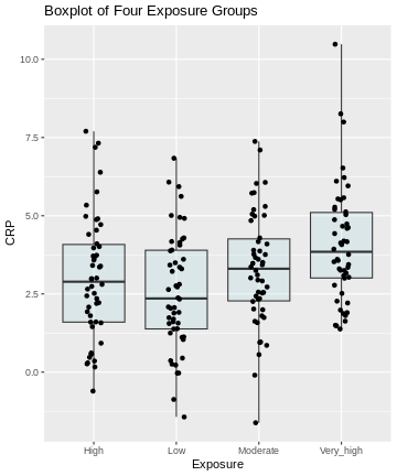
Here, we visualize the data as a boxplot, together with the individual data points:
R
# Visualize the data
ggplot(exp_data, aes(x = Exposure, y = CRP)) +
  geom_boxplot(coef = 5, fill = "lightblue", alpha = 0.25) +
  geom_point(position = position_jitter(width = .1)) +
  labs(title = "Boxplot of Four Exposure Groups")
Pairwise comparisons
In the above example:
- How many pairwise comparisons are possible?
- What is a suitable test for making these comparisons?
- If we choose \(\alpha =0.05\), what is the probability of seeing at least one significant difference, if in fact all differences are 0?
- 6 pairwise comparisons are possible.
- t-test
- \(1-(0.95)^6 \approx 0.26\)
Defining the question
Generally, from the above plot, as the exposure level increases from low to very high, we might expect to see a corresponding increase in the median exposure level and higher median C-reactive protein (CRP) values.
On this type of data, we can run different types of analyses, depending on the question we ask. Let’s look at two different scenarios:
Scenario 1: This is an exploratory analysis. We are interested in finding out whether there is any difference between the four exposure groups at all.
Scenario 2: We have one or more particular exposure groups of interest, which we like to compare to the low exposure group. In this case, the low exposure group serves as a reference.
Scenario 1: ANOVA
In this scenario, we’re basically comparing all against all.
Our null hypothesis is that there are not any differences in CRP amounts in the different groups. From the challenge above, we learned that 6 individual comparisons are not unlikely to produce at least one false positive. In case that there are no differences at all, this probability is estimated to be \(P=0.26\).
Recall that in this situation, we like to control for the family-wise error rate. Our null hypothesis is that there’s nothing going on at all, and once we reject the null for one of our individual comparisons, we also reject this overall null hypothesis.
In this kind of situation, the ANOVA F-test is the method of choice. It is a method that
- is used to compare means between different groups and
- controls for the family-wise error rate.
- It’s applicable when the data points are normally distributed around the group means and the variances are similar among the groups. This appears to be the case in our example.
In general, a one-way ANOVA for \(t\) groups tests the null hypothesis:
\[H_0: \mu_1 = \mu_2 = ... = \mu_t,\] where \(\mu_i\) is the mean of population \(i\).
The alternative hypothesis is:
\[H_A: \mu_i \neq \mu_j \text{ for some i and j where i}\neq \text{j}\]
For this, we use an F-statistic:
\[F= \frac{\text{between group variance}}{\text{within group variance}}\] \(F\) becomes large, if the groups differ strongly in their group means, while the variance within the groups is small. ANOVA is closely related to the t-test. In fact, if we perform an ANOVA on a data set with two groups only, it is equivalent to performing a t-test. For more details on ANOVA, see the PennState online materials.
We can perform an ANOVA in R as follows:
R
anova_result <- aov(CRP ~ Exposure, data = exp_data)
summary(anova_result)
OUTPUT
             Df Sum Sq Mean Sq F value  Pr(>F)
Exposure      3   60.8  20.268   5.754 0.00086 ***
Residuals   196  690.4   3.523
---
Signif. codes:  0 '***' 0.001 '**' 0.01 '*' 0.05 '.' 0.1 ' ' 1
The ANOVA output above shows statistically significant differences among the means of the four exposure groups. We therefore reject the null hypothesis of equal means.
Post-hoc tests
ANOVA alone does not tell us which specific groups differ significantly from each other. To determine this, we need to conduct further analysis. Post-hoc tests are follow up procedures, used to compare pairs of groups in order to identify where the differences lie. These tests provide more detailed information about which specific group means are different from each other.
Parametric methods, such as Tukey’s HSD, are used when assumptions of
normality and homogeneity of variance are met. Non-parametric methods,
such as pairwise Wilcoxon tests, are suitable when data do not meet the
assumptions of parametric tests. In R, performing pairwise comparisons
is straightforward using built-in functions and packages. We perform a
Tukey post-hoc test using TukeyHSD() to determine which
specific exposure group means differ significantly from each other.
R
tukey_result <- TukeyHSD(anova_result)
tukey_result
OUTPUT
  Tukey multiple comparisons of means
    95% family-wise confidence level

Fit: aov(formula = CRP ~ Exposure, data = exp_data)

$Exposure
                         diff        lwr       upr     p adj
Low-High           -0.4233920 -1.3960536 0.5492695 0.6727404
Moderate-High       0.3006174 -0.6720442 1.2732790 0.8539510
Very_high-High      1.0854145  0.1127530 2.0580761 0.0219956
Moderate-Low        0.7240094 -0.2486521 1.6966710 0.2193881
Very_high-Low       1.5088066  0.5361450 2.4814681 0.0004795
Very_high-Moderate  0.7847971 -0.1878644 1.7574587 0.1597266
The results provide pairwise comparisons of group means including
-
diff: the estimated difference between the two groups - the lower (
lrw) and upper (upr) bounds of a 95% family-wise confidence interval and -
p adj: the adjusted p-value which can be used to control for the FWER.
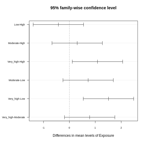
You often read that the Tukey procedure calculates simultaneous confidence intervals, which implies that the confidence intervals are dependent on how many comparisons we make. They grow (more uncertainty), the more comparisons we make, and they can also be used to determine whether two groups are significantly different. In the plot below, each comparison has an estimate, and a confidence interval. We call the difference significant with a 95% family-wise confidence level, if the confidence interval excludes 0.
R
library(multcompView)
par(mar=c(5,6,4,1)+1)
plot(tukey_result,
     las=1,
     cex.axis=0.7)
Interpreting Pairwise Comparison Results
Adjusted p-values reflect the probability of observing a given result (or more extreme) under the assumption that all null hypotheses are true, while accounting for the number of comparisons made. Here, we interpret pairwise comparison results with adjusted p-values from the Tukey test by assessing whether the adjusted p-value is less than the chosen significance level (α) (0.05). If the adjusted p-value is below the significance level, we conclude that the observed difference is statistically significant after correcting for multiple comparisons.
In our example above, we observe significant differences in CRP level
- between the exposure groups
very_highandhigh - between the exposure groups
very_highandlow
Consistent with that, the respective confidence intervals of these two comparisons exclude zero.
Scenario 2
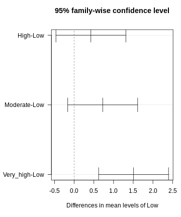
In the second scenario, we aim to determine risk areas of increased CRP concentration. Our control are low exposure regions, and we aim to find out which of the other groups differ significantly from the control in terms of CRP concentration, which classifies them as risk regions.
If this is our question, in theory, we don’t need all six comparisons. We just want to compare each group to the control. In biology, this is a common scenario. We might have a small screen, where we test several substances against a control, and need to determine which of these has an effect. In this scenario, Tukey is overly conservative, because it corrects for more tests than we actually like to perform. We can, however apply the Dunnett procedure, which
- controls for the FWER
- in a scenario where we’d like to compare a number of groups to a control.
We can run the Dunnett test in R by using the function
DunnettTest. As input, we supply
-
x: a numeric vector of data values, or a list of numeric data vectors -
g: a vector or factor object giving the group for the corresponding elements of x -
control: the level of the control group against which the others should be tested
R
library(DescTools)
dunnett <- DunnettTest(x =exp_data$CRP,
            g= exp_data$Exposure,
            control = "Low")
dunnett
OUTPUT
  Dunnett's test for comparing several treatments with a control :
    95% family-wise confidence level

$Low
                   diff     lwr.ci   upr.ci    pval
High-Low      0.4233920 -0.4652856 1.312070 0.53610
Moderate-Low  0.7240094 -0.1646682 1.612687 0.13711
Very_high-Low 1.5088066  0.6201290 2.397484 0.00023 ***

---
Signif. codes:  0 '***' 0.001 '**' 0.01 '*' 0.05 '.' 0.1 ' ' 1
R
par(mar=c(5.1, 7.1, 4.1, 1.1))
plot(dunnett, las=1)
Discussion
Why can’t we just run t-tests and then apply Bonferoni?
This would not be wrong. It doesn’t produce confidence intervals though. It’s sometimes a matter of convention.
Be honest!
In some cases, Dunnett is the way to go. But take a minute and think about whether you’re not interested in the other comparisons as well. For instance, when studying air pollution in different groups, you might also be interested in whether there are differences between moderate and high exposure. The fact that we don’t see large differences between those two groups in the data is not a good reason for leaving out this comparison!
Pretty figures
In publications, you often find p-values plotted next to the comparison in a figure. These plots can be produced in R.
Publication-ready plots
The R package ggpubr comes with the promise of producing
publication-ready plots. Let’s explore some of the functions and
practice our plotting skills. We use the PlantGrowth data
set.
- Explore the data set. Which variables are there?
- Use the following template to create a meaningful plot, comparing
the groups in the data set using ANOVA. You can look up the function
stat_compare_meansin the R help section.
R
library(ggpubr) # load the required library

PlantGrowth %>%
  ggplot(aes(x=, y=))+
  geom_jitter(width=0.1)+ # feel free to replace by, or add, another type of plot
  stat_compare_means()
Consult
?PlantGrowth, or checknames(PlantGrowth). The data set compares the biomass (weight) in a control and two treatment conditions.
R
library(ggpubr)
PlantGrowth %>%
  ggplot(aes(x=group, y=weight))+
  geom_jitter(width=0.1)+
  stat_compare_means(method="anova")
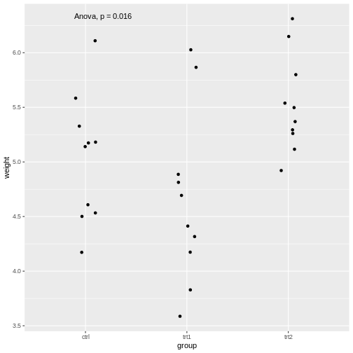
The stat_compare_means function infers the comparisons
to be made from the x and y that we supplied
in the aes.
We saw that the stat_compare_means function allows you
to conveniently add the p-value of an ANOVA in the plot. We can also add
the p-values for individual comparisons:
R
PlantGrowth %>%
  ggplot(aes(x=group, y=weight))+
  geom_jitter(width=0.1)+
  stat_compare_means(method="anova", label.y = 7)+
  stat_compare_means(comparisons=list( c("ctrl", "trt1"), c("ctrl", "trt2")), method="t.test")
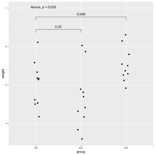
Explanations on the code above:
- The setting
label.y = 7shifts the result of the ANOVA to a height ofweight=7, so it won’t overlap with the individual results. - If we self-define the comparisons, we can do this via the
comparisonsargument by supplying a list of the comparisons to be made.
For more examples with the package, look up this page.
p-value hacking and data snooping
We learned in this lesson that performing a series of tests increases the chances of having at least one false positive. Therefore, it is important to be transparent about which tests were conducted during a study. If we run a large screen and reported only the tests that came out as hits, we’re skipping the type-I error control, and for someone else it is not comprehensible how much the results can be trusted. In fact, we could perform a screen of 1000 biological samples, where there are no true positives. Still, if we run each test at \(\alpha=0.05\), we would have around 50 hits, which are all false positives. The practice of analyzing data extensively, testing multiple hypotheses, or making comparisons until finding a statistically significant result or an interesting pattern, is called p-value hacking.
But even if this is not your intention, you may still sometimes be tempted to snoop in the data, which is a more subtle way of increasing type I error.
Reconsider the air pollution example above:
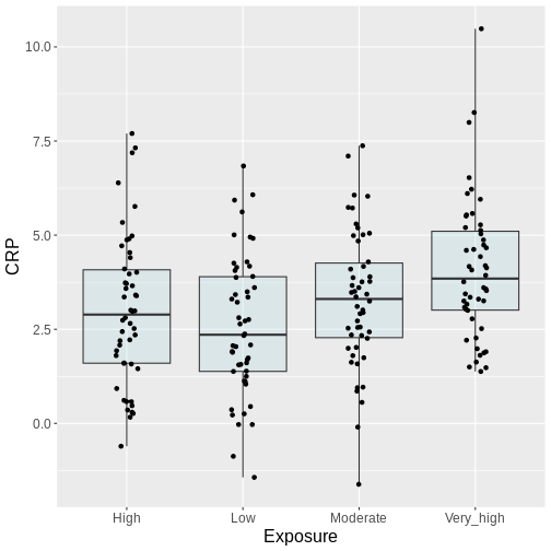
In this example, we might visually inspect our plot, and decide to perform only the comparison between very high and low. Why? Because it looks most promising. With only one test performed, there is also no possibility to perform correction for multiple testing, which may seem sound, while in reality, you performed all the pairwise comparisons by eye, without correcting for them. Therefore, unless you pre-specified one particular test before you inspected the data, all tests should be performed and reported. Otherwise, this approach will lead to inflated Type I error rates.
Additional resources
For further reading and hands-on practice with pairwise comparisons in R, refer to R documentation on pairwise comparisons, Applied Statistics with R and book by Oehlert 2010 resources.
Inline instructor notes can help inform instructors of timing challenges associated with the lessons. They appear in the “Instructor View”
