The binomial distribution

Overview

Questions

• What is the binomial distribution?
  
• What kind of data is it used on?

Objectives

• Explain how the binomial distribution describes outcomes of counting.

The binomial distribution is what we have just seen in the example: We use it when we have a fixed sample size and count the number of “successes” in that sample. Examples are:

• how many locations in the genome carry a mutation
• the number of cells within a sample that show a certain phenotype
• how many patients out of 100 have a certain disease
• how many out of 10 frogs are light green

The binomial model has two parameters, which means the probabilities for the individual outcomes depend on two things: - \(n\) is the number of trials, or frogs, or patients, and it’s fixed. - \(p\) is the success probability.

Then the probability of observing \(k\) successes out of \(n\) draws (for example \(k=4\) light coloured frogs out of \(N=10\)) can be described by this formula:

\[P(X=k) = {n\choose k}p^k(1-p)^k\]

You don’t have to remember this piece of math – it’s just to make the point that you can calculate the probability of an event that is modeled with the binomial distribution, if you know the success probability \(p\) and the number of trials \(n\), i.e. the parameters.

Callout

In the binomial we just define a particular outcome as success, for example a light-coloured frog, or a patient with disease, even though that may not be a favourable outcome.

Here is what the distribution looks like for a success probability of 0.3 and a sample size of 10.

The binomial distribution

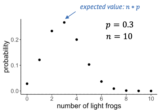
The expected value of the binomial is \(n \times p\), which is quite intuitive: If we catch 10 frogs and the probability of being light-green is 0.3, then we expect to catch 3 light-green frogs on average.