The cumulative distribution function

Overview

Questions

• What is the empirical cumulative distribution function?

Objectives

• Demonstrate the cumulative distribution function with an example.

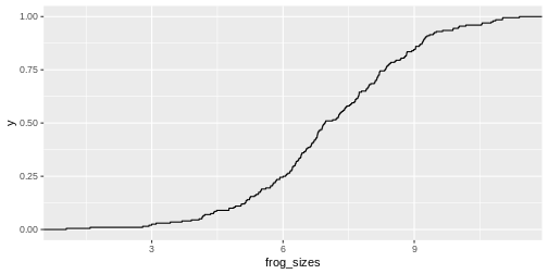
The cumulative distribution is the integral of the distribution, and thus the empirical cumulative distribution is the integral of the histogram. It gives you the percentage of values that are smaller than a certain value.
We can visualize it with stat_ecdf in ggplot2.

R

data.frame(frog_sizes) %>% 
  ggplot(aes(x=frog_sizes))+
  stat_ecdf()

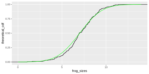
As for the histogram, you could calculate the expected values for the cumulative distribution and add them to the plot:

R

sizes <- seq(0,14,.5)
theoretical_cdf <- pnorm(sizes, mean=7, sd=2)

data.frame(frog_sizes) %>% 
  ggplot(aes(frog_sizes)) +
  stat_ecdf()+
  geom_line(data=data.frame(sizes,theoretical_cdf), aes(sizes, theoretical_cdf),colour="green")

Off this plot you can read for a frog size of \(x\) (e.g. 7cm), that about 50% of the values are smaller than this value. So this is really just another way to display the histogram.

Note

The procedure above was shown for demonstration purposes. We will not practice overlaying empirical and theoretical distribution functions with ggplot, because in the next episode, we’ll introduce a tool that does the work for you.