Our first test: Disease prevalence

Estimated time: 17 minutes

Overview

Questions

• What is the null distribution?
• How can we use the null distribution to make a decision in hypothesis testing?
  
• How can we run a hypothesis test in R?

Objectives

• Give an example for a simple hypothesis test, including setting up the null and alternative hypothesis and the corresponding null model, and decision making.
  
• Demonstrate how p-values can be calculated from either cumulative probabilities or the .test functions in R.

Throughout the next episodes, we consider a research project where we want to find out whether the prevalence of a disease in a test group is different from the population average. We’ll conduct a very simple test to answer that question.

Example: Disease prevalence

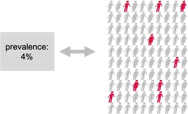
Suppose There is a disease with a known prevalence of 4%. This means, 4% of the whole population have this disease. Now you are interested in whether a certain pre-condition, let’s say overweight, or living in a certain area, changes the risk of getting the disease. You take 100 persons with this precondition and you check the disease prevalence within the test group. 9 out of the 100 test persons have the disease.

Null and alternative hypothesis

This is how we can formalize the hypotheses: Our null hypothesis is the “boring” outcome. If there is nothing to see in the data, then the prevalence in the test group is also 4%, just as in the whole population. We want to collect evidence against this hypothesis. If we have enough evidence against the null, we reject it, and accept the alternative hypothesis that the prevalence in the test group differs from 4%. This test is so easy, because the null model is simply the well-known binomial distribution with a sample size of 100 and a probability of 4%:

\[ H_O: X \sim Bin(N=100, p=0.04)\]

The null distribution

We can look at this distribution:

The null distribution

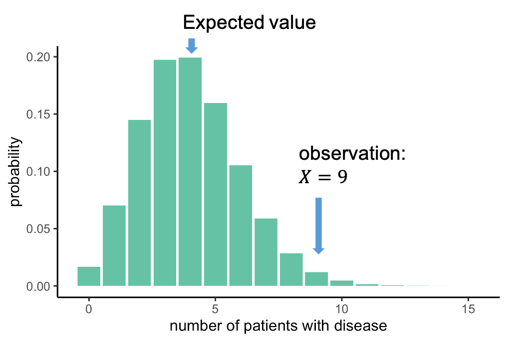
It gives us the probabilities of seeing \(X\) cases out of 100 with the disease, given that each individual has a probability of 4% of having this disease. This distribution peaks at 4 out of a 100, which makes sense: You expect to see around 4 out of a 100 when the probability is 4%. We, on the other hand, observed 9 out of a 100. Now we can ask: How likely is it to see an event at least as extreme as 9 out of 100, assuming the null hypothesis, and thus the distribution above, is true. In this case, the probability of observing 9 or more persons with the disease is 0.019, this is rather unlikely, and we will conclude that the null hypothesis is likely false.

Decision: Do we reject the null hypothesis?

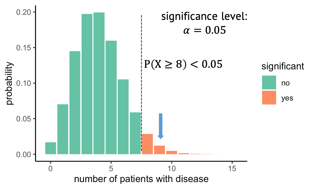
At what probability should you decide to reject the null hypothesis? This choice is rather arbitrary. It depends on how sure you want to be that there is really something to see in the data set. A wide-spread convention is to call the result significant if the probability under the null hypothesis is smaller than 5%. We say that you choose a significance level alpha of \(\alpha=5 \%\). In our example, with a significance level of 5%, all observations above 8 out of 100, shown in red, would be called significant.

The null distribution

Recap

Here is what we have just seen:

• In a test group of persons with a precondition, 9 out of 100 have the disease of interest.
  
• We compare to a known prevalence of 4%, that means 4% of the entire population have the disease, when not distinguishing between persons with and without the precondition.
  
• We want to know whether the observed 9 out of 100 are significantly different from 4%. The null hypothesis thus is that they are not.
• The alternative hypothesis is that the prevalence in the test group differs from 4%.
  
• As we have 100 cases and a binary outcome (disease or no disease), a suitable null model is a binomial distribution with \(n=100\) and success probability \(p=0.04\).

Binomial test in R

R is very convenient for calculating probabilities under different distributions, and also has functions for the common statistical tests.

As a reminder, functions in R that calculate numbers for the binomial distribution all end with binom, and the prefix specifies what to calculate:
- dbinom: density
- pbinom: cumulative distribution function (percentage of values smaller than)

For example, you can calculate the probability of observing 5 persons out of 100 with a disease, given a prevalence of 4%:

R

n = 100 # number of test persons
p = 0.04 # given prevalence
dbinom(x=5, size=n, prob=p)

OUTPUT

[1] 0.1595108

Challenge: Binomial test

1. Can you perform the test demonstrated above, using pbinom? For this, you need to calculate the probability of observing 9 or more persons with a disease out of 100, given a “null prevalence” of 4%.

2. Look up binom.test. This function performs a binomial test – which is what you have just done manually by calculating a binomial probability under a null hypothesis. Use this function to perform the test. Do you get the same result as with pbinom?

You can look up the function as follows:

R

help(binom.test)

Show me the solution

1. Calculate the probability as follows:

R

pbinom(q=8, size=100, prob=0.04, lower.tail=FALSE)

OUTPUT

[1] 0.01899192

Note: We use q=8, because if lower.tail=FALSE, the probability \(P(X>x)\) is calculated. Check help(pbinom) for this.

2. Using binom.test:

R

binom.test(9,100,p=0.04)

OUTPUT

	Exact binomial test

data:  9 and 100
number of successes = 9, number of trials = 100, p-value = 0.01899
alternative hypothesis: true probability of success is not equal to 0.04
95 percent confidence interval:
 0.0419836 0.1639823
sample estimates:
probability of success 
                  0.09 

Discussion

Before we continue to the next episode, I have to tell you that something is very wrong (conceptionally) with the test we just performed.

Please take a minute…

… and think about what the initial alternative hypothesis was, and whether this is in line with what we calculated.

(Image: Wikimedia)